Anonymous submission · under review

ResiCLAP: Semantic-Preserving Residual Enhancement for Fine-Grained Impact Sound Retrieval

CLAP retrieves the right kind of sound, but not the right one. ResiCLAP adds bounded residuals to a frozen CLAP embedding so that fine-grained acoustic and temporal detail becomes searchable — without disturbing the pretrained semantic structure, and without leaving the single-vector retrieval setup.

Listen to retrieval results See the results How it works

The problem

A sound designer searching for a “metal impact” gets hundreds of results that are all, correctly, metal impacts. What separates a usable take from an unusable one is finer: how bright it is, how sharp the attack is, how long it rings. These properties are category-relative — a bright metal impact and a bright wooden impact occupy very different absolute spectral ranges — and global audio–language embeddings tend to emphasise between-category separation while under-expressing this within-category variation.

Frozen backbone

Both CLAP encoders stay frozen. Only two small residual branches and their gates are trained.

Bounded residuals

Each residual is projected off the frozen embedding and clipped to a fixed radius, so the output is a bounded rotation of the original vector.

Drop-in retrieval

The output is still one normalised 512-d vector. Cosine search over an unmodified CLAP index works unchanged.

Headline result

Model	Fine-grained R@1	Fine-grained nDCG@10	Clotho R@1	FSD50K R@1
Frozen CLAP	0.208	0.232	0.320	0.375
FineLAP	0.208	0.216	–	–
Two-stage property scoring	0.417	0.368	–	–
ResiCLAP (full)	0.500	0.450	0.338	0.450

Fine-grained retrieval: 400 held-out RealImpact test recordings, 24 text queries, mean over three seeds. Broad retrieval: 200 Clotho and 200 FSD50K examples. Broad retrieval is not reported for FineLAP, which modifies the text encoder, nor for two-stage scoring, which keeps the CLAP index and only rescores property queries.

nDCG@10 on fine-grained retrieval rises from 0.232 to 0.450 — a gain of +0.218 (95% CI [0.117, 0.321]) — while Clotho and FSD50K retrieval stay at or above frozen-CLAP levels.

At a glance

<1% of CLAP parameters trained

+0.218 fine-grained nDCG@10 over frozen CLAP

400 held-out test recordings

24 evaluation text queries

Evaluation data

Fine-grained retrieval is evaluated on RealImpact, a set of real recordings of everyday objects struck at controlled points and captured by a dense microphone array. Because every recording carries its object, material, strike point and microphone position, it supports queries that differ only in acoustic detail rather than in category.

Training and test splits are disjoint by object, so no object heard at training time appears at test time. The held-out pool used throughout this site contains 400 recordings of 5 unseen objects — Mug (ceramic), Bin (plastic), Flowerpot (small ceramic), Vase (wood), Spatula (metal) — each struck at 5 points and recorded across 4 microphone distance rings and a range of angles.

Attribute supervision is category-relative: brightness, attack and decay targets are standardised within each material, so “bright” means bright relative to other sounds of that material rather than bright in absolute spectral terms. Semantic retention is measured separately on Clotho and FSD50K, which the model never trains on as a retrieval target.

Dataset curation

Fine-grained supervision needs pairs that differ in one attribute and nothing else. RealImpact supplies the recordings; the curation pipeline supplies the contrast.

1. From recordings to factor measurements

Objects are grouped into materials by name, and every clip is analysed at 48 kHz after onset detection (first point where a 5 ms moving-average envelope reaches 10% of its peak). Three scalar factors are measured:

Factor	Measured quantity	Target value
Brightness	Spectral centroid of the Hann-windowed active region (up to 1 s after onset)	`log10(centroid + 1)`
Attack	Rise time from onset to 90% of the local envelope peak, within a 100 ms window	`-log10(t₉₀ + 1/f_s)`
Decay	T20 from the backward energy-decay curve, noise floor subtracted	`log10(T20 + 1e-4)`

Higher target means brighter, sharper, or longer-ringing respectively. Clips whose decay curve never crosses −20 dB before the recording ends are marked censored and excluded from decay supervision.

2. Category-relative targets

A ceramic bowl is brighter than a wooden block in absolute terms even when it is the dullest ceramic in the set, so absolute thresholds would simply re-encode material identity. Each factor is therefore standardised within its material, using statistics computed on the training split only. A clip below the 45th percentile of its material's training distribution is labelled low, above the 55th high, and otherwise middle. Splits are assigned at the object level with a deterministic seeded hash, stratified by material, so no object and no normalisation statistic ever crosses from training into test.

3. Controlled DSP variants

Natural recordings alone rarely give two clips of the same object differing in exactly one attribute. Each reference clip is therefore processed into candidate variants pushed toward the low and high end of its own category. Every candidate is RMS-matched back to the reference and peak-limited at 0.98, so loudness can never be the cue that separates them.

Variant	Transform	Parameter sweep
Brighter / duller	Second-order high-shelf biquad, cutoff 2 kHz	`±3, ±6, ±9, ±12 dB`
Sharper attack	Time-warp of the attack segment, `t → t^w`	`w = 0.5, 0.25, 0.125, 0.0625`
Sharper attack	Transient boost `1 + s·exp(−t/2ms)` over the first 40 ms	`s = 1, 2, 4`
Softer attack	Time-warp of the attack segment	`w = 1.5, 2, 2.5, 3.5, 5`
Softer attack	`sin²` onset ramp	`5, 10, 20 ms`

The sweep is not a fixed setting applied blindly — all candidates are generated, measured, and then filtered by the gates below.

4. Acceptance gates

A candidate is kept only if it clears every gate. The strength that survives therefore varies per clip, which is the point: a dull ceramic needs a different push than an already-bright one.

Headroom

The original must have room to move — below the category's 90th percentile to brighten, above the 10th to dull.

Direction

The re-measured factor must actually move the intended way. Intent is never assumed from the parameter.

Plausibility

The result must land inside the 1st–99th percentile of real clips of that material and object type.

Leakage

The other two factors must barely move — the constraint that makes the pair single-attribute.

Leakage tolerances are asymmetric, because brightening is more likely to disturb a measured attack than the reverse:

Variant type	Max Δbrightness	Max Δattack	Max Δdecay
Brightness variants	—	0.15	0.15
Attack variants	0.10	—	0.15

Among surviving candidates, the one closest to the category's 25th (low) or 75th (high) percentile wins, scored as |measured − target| / (q95 − q05) + 0.1 × leakage. Finally, each accepted variant must keep a frozen-CLAP cosine of at least 0.85 to its original, so no variant drifts far enough to change what the clip is a recording of.

5. Why decay has no synthetic variants

Decay is supervised only by natural recordings. Synthetic decay variants were generated in an earlier pass — exponential rescaling of the tail with a fade — and then discarded, because lengthening or truncating a ring changes how bright and how sharp the clip measures as well, and the processed audio failed the semantic-preservation check. Rather than train on supervision we could not keep clean, decay pairs are drawn from natural RealImpact groups whose ring time already differs under controlled geometry.

This is a deliberate asymmetry rather than an oversight, and it is worth stating plainly: brightness and attack benefit from controlled augmentation, decay does not.

Method

ResiCLAP treats the frozen CLAP embedding as a fixed semantic anchor and learns only bounded corrections around it.

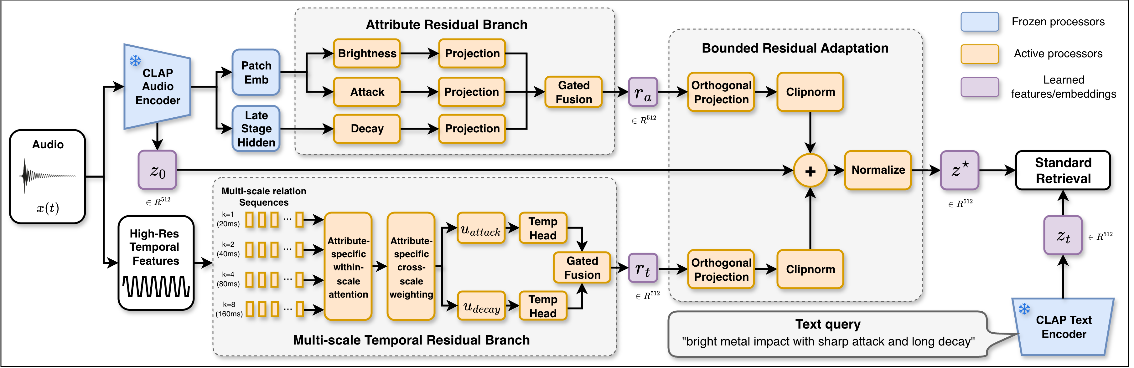
Overview of ResiCLAP. Blue blocks are frozen, orange blocks are trained, purple blocks are embeddings. Both CLAP encoders stay frozen. An attribute residual branch reads patch and late-stage hidden states to recover brightness, attack and decay evidence, while a multi-scale temporal relation branch reads high-resolution features at four offsets. Each residual is projected orthogonally to the frozen embedding z₀ and clipped in norm, then both are added back and re-normalised into a single enhanced embedding z^★ that is matched against the unmodified CLAP text embedding by ordinary cosine retrieval.

1. Attribute residual branch

Probing the frozen HTSAT encoder shows that intermediate layers expose fine-grained attributes more strongly than the final global embedding. We read three of them directly:

Attribute	Source representation	Dimension
Brightness	patch spectral-band features	384
Attack	patch onset features	96
Decay	stage-3 tail features	768

Each is projected to 512-d by a two-layer MLP (hidden width 128, LayerNorm, GELU) and the three projections are merged by a learned sigmoid gated fusion. Every gate is initialised to −2, so each branch starts with a small contribution and has to earn its influence during training.

2. Multi-scale temporal residual branch

CLAP's own frame stride is too coarse for transient detail, so this branch reads the waveform at higher resolution. From a 1.5 s window beginning 100 ms before onset we extract 5 ms log-mel frames plus envelope, spectral-flux and relative-time features, standardise them, downsample to 20 ms steps and project to 64-d states.

Temporal evolution is then modelled explicitly as relations between time steps at four offsets — 20, 40, 80 and 160 ms — so the branch sees both short transients and longer evolution. Attribute-specific attention summarises each scale, and a second attribute-specific weighting combines the four scales.

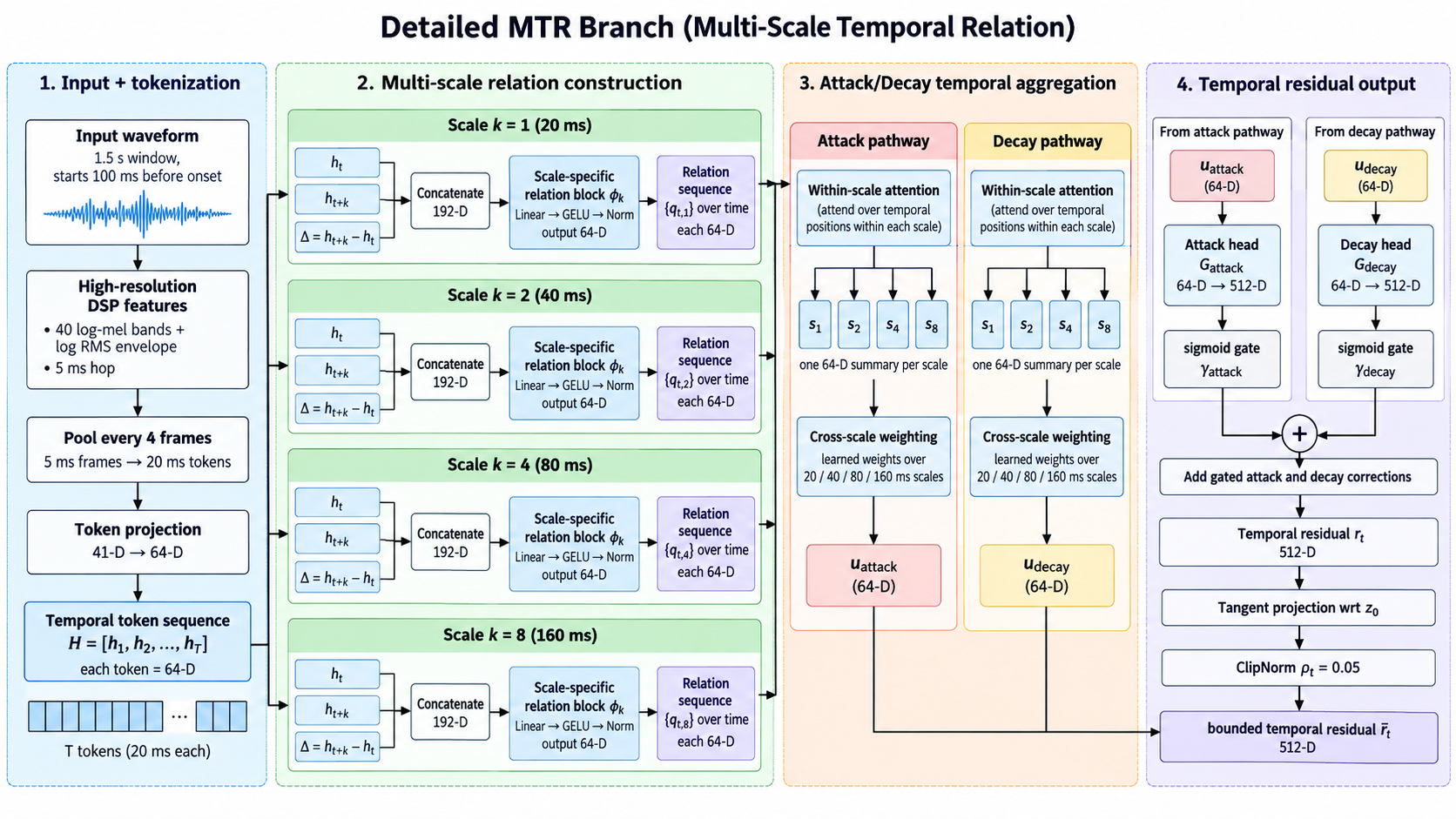
The multi-scale temporal relation branch. Relation sequences are formed over four temporal offsets, summarised by attribute-specific within-scale attention, then combined by attribute-specific cross-scale weighting before being mapped into the CLAP space.

3. Bounded residual adaptation

This is the part that keeps CLAP intact. Each residual is first projected orthogonally to the frozen embedding, then clipped to a fixed radius:

r̅_b = ClipNorm( r_b − ⟨r_b, z₀⟩ z₀ ; ρ_b ), b ∈ {a, t}

with ρ_a = 0.20 for the attribute residual and ρ_t = 0.05 for the temporal residual. The bounded residuals are added to the anchor and re-normalised:

z^★ = ( z₀ + r̅_a + r̅_t ) / ‖ z₀ + r̅_a + r̅_t ‖₂

Because the residuals are orthogonal to z₀ and bounded, the enhanced embedding is a rotation of the original by at most about 14°. Our ablation shows it is the magnitude bound, not the orthogonal projection, that does the work of preserving semantic structure — see the trade-off analysis.

4. Training objective

The bound controls how far the embedding may move; the objective decides what the movement should encode. Two groups of terms are combined:

Fine-grained learning

Prompt classification aligns the enhanced embedding with its material–attribute description.
Smooth-L1 regression predicts the category-relative attribute value.
Pairwise ranking preserves the relative ordering between sounds.

Semantic preservation

Cosine anchor penalises deviation from z₀.
Semantic contrastive keeps audio–text alignment on general audio.
Symmetric-KL distillation matches the frozen and enhanced audio–text similarity distributions.

Training setup

Setting	Value
Backbone	LAION-CLAP `clap-htsat-fused` (frozen)
Trained parameters	residual branches and gates only
Optimiser	AdamW, lr 1e−4, weight decay 1e−4
Gradient clipping	global norm 5.0
Epochs	100
Alignment temperature	0.07
Attribute bound ρ_a	0.20
Temporal bound ρ_t	0.05
Seeds	7, 17, 27